SUNDIALS and hypre: Exascale-Capable Libraries for Adaptive Time-Stepping and Scalable Solvers

By Rob Farber, contributing writer

Scientific computing often involves applying sophisticated mathematical techniques to systems of equations that reflect or model something of interest in the real world. Part of the magic of mathematics is that the same or similar mathematical techniques can work with systems of equations for wildly disparate physical phenomena, such as the dynamics of change in an animal population, , the behavior of plasma in unexplored physics regimes in the ITER fusion reactor, or subsurface fluid flows for carbon sequestration.

For this reason, numerical libraries have a significant impact on scientific computing as algorithmic advances can improve the speed and accuracy of many modeling and simulation packages. These libraries also act as the gateway middleware that enables many applications to run on state-of-the-art hardware and to leverage performance-enhancing features such as mixed-precision arithmetic.

In meeting these and other obligations, the mathematicians and developers of numerical libraries must follow good programming practices—starting with the API used by the application programmers and continuing through all aspects of the code from the build process to the regression, verification, and continuous-integration test suites that verify correct operation on all supported hardware platforms. Great care must be taken to ensure that the library does not contain mathematical, numerical, or programming errors that can corrupt or introduce non-physical artifacts into a computer simulation—regardless of the hardware platform or device utilized.

Two Complementary Libraries in the ECP SUNDIALS–Hypre Project

The SUite of Nonlinear and DIfferential/ALgebraic equation Solvers (SUNDIALS) and hypre are two complementary but distinct numerical libraries funded through the Exascale Computing Project (ECP) project.

Both libraries have been around for decades. The reliance of exascale systems on GPU-accelerated computing requires that both libraries reevaluate their algorithms, API, and code base to support these devices. GPUs very efficiently implement the single instruction, multiple data (SIMD) and single instruction, multiple thread (SIMT) execution models. The caveat is that these execution models impose performance restrictions on some types of calculations. Particularly troublesome for mathematical libraries is a limitation on nested conditional operations that can incur an order of magnitude slowdown.[1]^,[2] The successful adaptation of the methods in these libraries provides enhanced capabilities that align with the ECP mission to create “a software stack that is both exascale-capable and usable on US industrial- and academic-scale systems.”[3] Recent benchmark results from the Crusher and Spock systems, which are early access test-bed systems for the Frontier supercomputer,[4]^,[5] demonstrate that both libraries can support production runs on the Frontier exascale system after it passes its ready-for-production acceptance tests. Crusher and Spock contain identical hardware to the Frontier system and similar software.

SUNDIALS

The SUNDIALS project—led by Carol Woodward (Figure 1), PI and distinguished member of the technical staff at Lawrence Livermore National Laboratory (LLNL)—focuses on delivering adaptive time-stepping methods for dynamical systems.

Sundial Contributors, Carol Woodward (top-left), and active contributors Cody Balos (top-right), David Gardner (bottom-left), and Daniel Reynolds (bottom-right).

Figure 1. Carol Woodward (top-left), and active contributors Cody Balos (top-right), David Gardner (bottom-left), and Daniel Reynolds (bottom-right).

Many numerical problems can be expressed as ordinary differential equations (ODEs). The term ordinary is used to indicate functions of one independent variable and the derivatives of those functions. This contrasts with a broad class of equations referred to as partial differential equations (PDEs) which are used to describe change with respect to more than one independent variable.[6] PDEs are often solved using a method of lines approach which first applies a spatial discretization leading to a system of ODEs. Scientists use hypre (discussed below) to solve the spatial dependencies in many types of PDE systems.

Scientists use ODEs and PDEs to describe the dynamics of changing phenomena, evolution, and variation in a system. Often, quantities are defined as the rate of change with respect to time, where time is considered the independent variable. Additionally, scientists utilize time-step integrators to examine the evolution of the system over time. Consider the SUNDIALS tutorial example, which models the transport of a pollutant that has been released into a flow in a 2D domain. SUNDIALS is used to determine both where the pollutant goes, and when it has diffused sufficiently to no longer be harmful. The 3Blue1Brown video, “Differential equations, a tourist’s guide,” provides a quick overview for a general audience on why it is frequently easier for scientists to use differential equations (e.g., ODEs and PDEs) to model the dynamics of a system.

The adaptive time-stepping methods implemented in SUNDIALS promise both increased accuracy and faster time to solution. Woodward explained, “In many computational problems, the timescales change over time. Fixed time-step approaches can be very inefficient. To meet the accuracy needs of scientists while balancing run time, we need to adapt the timestep, thus allowing bigger time steps when timescales are longer and smaller time steps when timescales are shorter.” For more information, consult the SUNDIALS tutorial that explores fixed time-stepping compared with adaptive time-stepping and the impact on accuracy. These tutorials also reflect on the need for clear, concise, and solved tutorial problems to inform new users of the numerical package’s capabilities and benefits of the numerical package.

Woodward explained the need to support GPU devices and exascale computational capabilities: “Our code is buried inside other codes that need to run on exascale supercomputers. Because we are in the middle of the numerical software stack, our software must provide the flexibility to support data structures that utilize the GPU in a vendor-agnostic fashion. Fundamentally, SUNDIALS needs to give users the ability to call any solver they wish to use and enable them to use the most advanced systems available.” SUNDIALS can be accessed via the E4S, GitHub, Spack, the Extreme-scale Scientific Software Development Kit (xSDK), and a variety of third-party library distributions.[7] Python users can also access SUNDIALS in a variety of ways, such as Assimulo or the ODES scikit, and Julia users can access SUNDIALS through the Sundials.jl Julia package.

SUNDIALS gives users the ability to program for two fundamentally different use cases. Of interest is how the use cases map to GPUs:

SUNDIALS governs the overall time loop. Users can make this a GPU-based computation in which the code works on distributed data structures. Example applications include the Multiscale Finite Element Method (MFEM), the Energy Exascale Earth System Model (E3SM), the Exascale Additive Manufacturing project’s (ExaAM’s) Adaptive Mesh Phase-field Evolution (AMPE), and ExaAM’s Microstructure Evolution Using Massively Parallel Phase-field Simulations–Solid State (MEUMAPPS-SS).
SUNDIALS is used as a local time integrator. In this use case, application developers want to operate on several ODE systems simultaneously. Local time integrators enable programmers to leverage the GPU capabilities most efficiently. Example applications include AMReX, Nyx, PeleLM, PeleC, and PelePhysics.
- For example, every cell in a grid can issue a call to an ODE integrator. These integration operations are then batched and presented en masse to best make use of monolithic GPU parallelism. Monolithic refers to programming the GPU as a single SIMD device where all the computational units on the GPU (called streaming multiprocessors) run the same code and perform the same operations in lockstep.
- It is also possible to program the GPU by using a SIMT threading model in which each streaming multiprocessor runs a different thread of execution. which, unlike the monolithic model, gives the GPU the ability to perform many different tasks at the same time. Woodward observed that performance might benefit from using the SIMT model with multiple integrators but cautioned that this is very early-stage research.

SUNDIALS works with hypre and many other solver packages, such as Kokkos, SuperLU (including the distributed SuperLU_DIST interface), RAJA, Ginkgo, Matrix Algebra on GPU and Multicore Architectures (MAGMA), and Portable, Extensible Toolkit for Scientific Computation (PETSc). As noted on the LLNL SUNDIALS webpage, “the main numerical operations performed in SUNDIALS codes are operations on data vectors, and the codes have been written in terms of interfaces to these vector operations. The result of this design is that SUNDIALS users can relatively easily provide their own data structures to the integrators by telling the integrator about their structures and providing the required operations on them.”[8] This capability provides wonderful flexibility. For example, the SUNDIALS team recently added support for Kokkos data structures.

GPU support and compatibility means the SUNDIALS team has addressed key numerical library challenges identified in the 2021 ECP capability assessment report:[9]

Applications need both efficient integrators and ones that can interface easily with efficient linear algebra packages to solve subservient linear systems.
Integrators and their interfaces to both solver libraries and applications must be frequently updated to keep up with rapid advances in system architectures, such as the use case of the local time integrator, which requires solving many small systems of ODEs in parallel on GPUs.
ECP applications require assistance in incorporating new linear solvers underneath the integrators and in updating their interfaces to optimally use integrators on new platforms.

Recent Progress

The SUNDIALS team supports both CPUs and GPUs. To do so, SUNDIALS utilizes several back ends, such as CUDA, the Heterogeneous Interface for Portability (HIP), SYCL, Open Multi-Processing (OpenMP) offload, Kokkos, and RAJA (with CUDA, HIP, or SYCL back ends). For both flexibility and performance, the library leverages user-defined functions, optimized libraries, and optimized data structures and provides interfaces to accelerate performance according to machine type and external library availability:

Interfaces to MAGMA and the oneAPI Math Kernel Library (oneMKL) are provided for dense, batched, and lower-upper (LU) solvers.
An interface is provided to cuSOLVER for access to the NVIDIA batched sparse QR linear solver.
Iterative nonlinear and matrix-free linear (Krylov) solvers inherit GPU support from vectors and user-defined functions.
The SUNDIALS team is working with the Ginkgo project to test and interface their batched sparse linear solvers (through the xSDK) for CUDA-, HIP-, and Intel-based GPU systems.

Performance

SUNDIALS enables performance from laptops to exascale systems. Starting on the low end, Figure 2 shows the performance on a consumer-grade Intel Gen9 integrated GPU. According to Intel, these integrated GPUs approach teraflop performance and use a modular on-die architecture suitable for cellphones, tablets, laptops, and high-end desktops and servers.[10] The result can be high SUNDIALS performance, even on a laptop.

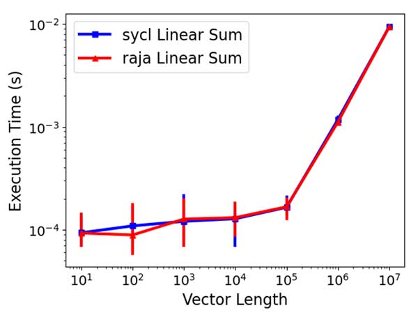
Figure 2. SYCL and RAJA vector timings on an Intel Gen9 integrated GPU. The performance of streaming operations (LinearSum) is equivalent to the native SYCL implementation and use of RAJA with a SYCL back end.

High-end discrete GPUs—a discrete GPU has its own memory system—and vendor-optimized libraries are also supported. Figure 3 shows that the SUNDIALS 2D diffusion benchmark problem runs ~1.5× faster with the AMD MI250X GPUs on Crusher (the same GPUs used in Frontier) than with the older AMD MI100 GPUs on Spock. The 1.5× speedup occurs with both the SUNDIALS ARKODE and CVODE integrators, but CVODE is faster overall.

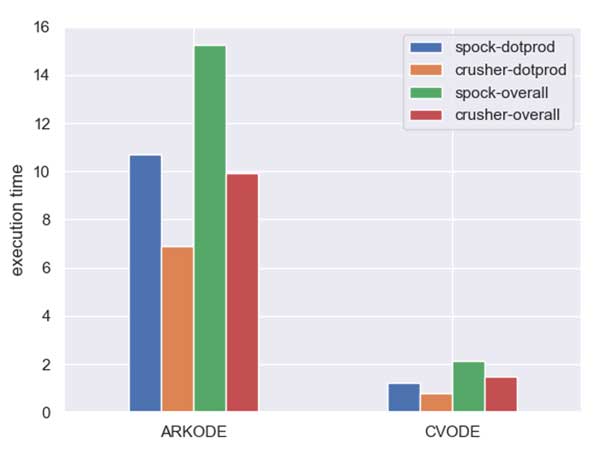
Figure 3. The SUNDIALS 2D Diffusion benchmark problem runs about 1.5× faster overall with the AMD MI250x GPUs on Crusher than on Spock with the older AMD MI100 GPUs.

Figure 4 illustrates the single-node speedup relative to the best performance on an AMD- or NVIDIA- accelerated compute cluster. On Summit, the maximum speedup (CPU time/GPU time) achieved is 8.8× overall, 10.8× for the linear solve, 7.2× for the dot product, and 30.9× for the right-hand side (RHS) time. On Spock, the maximum speedup (CPU time/GPU time) achieved is 3.8× overall, 3.9× for the linear solve, 2.1× for the dot product, and 7.8× for RHS.

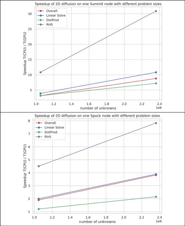
Figure 4. Top: Execution time of 2D diffusion benchmark problem on one node of Summit (i.e., CPU problems use all 40 CPU cores, and GPU problems use all 6 V100 GPUs). Bottom: Execution time of 2D diffusion benchmark problem on one node of Spock (60 CPU cores and 4 MI100 GPUs). The CVODE backward differentiation formula integrator is used with a preconditioned conjugate gradient (PCG) linear solver.

GPU-Agnostic Portability from Laptops to Supercomputers

Supporting such a wide range of devices and platforms required the adoption of good software practices. Out of necessity, the team automated the build process via the Spack build system. This automation helps prevent the team from being inundated with build issues. Essential to portability, benchmark problems that utilize CUDA, HIP, and RAJA have been incorporated into an LLNL GitLab continuous testing (CI) framework for automated performance testing. CI ensures that the library runs correctly on all supported platforms. Otherwise, code changes by the team or external factors, such as library updates at the site, could inadvertently introduce errors or performance issues.

The SUNDIALS team has also created optional interfaces to the Caliper library, which is a lightweight, Message Passing Interface (MPI)–aware, performance-profiling scheme that can be enabled at compile time. The graph shown in Figure 4 for example, was created with Caliper.

Support the ECP’s Exascale Computing Mission

SUNDIALS is currently used in PeleC, PeleLM, PelePhysics, Nyx, MFEM, AMPE (a stretch goal for the ExaAM project[11]), MEUMAPPS-SS, and AMReX, and this demonstrates the broad scope of applications.

Several of these applications are recent integration projects and reflect the success of the SUNDIALS integration strategy: regularly meeting with users, consulting with users as they add SUNDIALS interfaces, using Slack workspaces to quickly interact with users, participating in hackathons, and encouraging user feedback when possible (e.g., the breakout sessions during the ECP Annual Meeting).

Recent integration projects and benefits are as follows:

PelePhysics: Interfaces to CVODE and ARKODE are in place and include a new interface to MAGMA batched solvers.
PeleC: The team evaluated explicit integrator performance with various configurations on Summit. With their target chemistry mechanism and CVODE, absolute tolerances based on typical values provide 1.5× speedup vs. default tolerances. The team is currently testing with HIP and SYCL on Early Access Systems (EAS) systems.
PeleLM: CVODE is the default chemistry integrator. The interface to the batched, dense, direct MAGMA solvers can yield up to a 3× faster linear solve than a generalized minimal residual that is not preconditioned.
MFEM: The team developed a CUDA- and HIP-enabled interoperability example with xSDK.
Nyx: The team tested weak scaling on Summit with 1–13,824 GPUs (Figure 5), executed a full 1,024³ production Lyman-alpha run on Spock, and tested with HIP and SYCL on Spock and EAS systems.

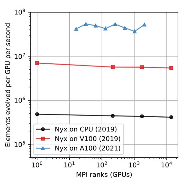
Figure 5. Nyx weak scaling on NVIDIA GPU systems vs. CPU OpenMP version (Summit CPUs), speed-up 13 – 14.5× over CPU. Performance on Perlmutter (Phase 1, subject to improvement) is now 100× over the pre-GPU (MPI+OpenMP) November 2021 version. (Figure and results courtesy of Jean Sexton.)

AMPE (ExaAM): AMPE supported the team as they interfaced with ARKODE to enable an implicit-explicit (IMEX) approach for moving mesh problems and treating the motion of the mesh explicitly. Initial results show greater efficiency with this approach.
MEUMAPPS-SS (ExaAM): The team interfaced ARKODE with a test application that solves the Cahn-Hilliard equation. An adaptive third order IMEX method provides a 10×–20× speedup in relevant error regimes (Figure 6). This test application runs successfully on Summit and Spock.

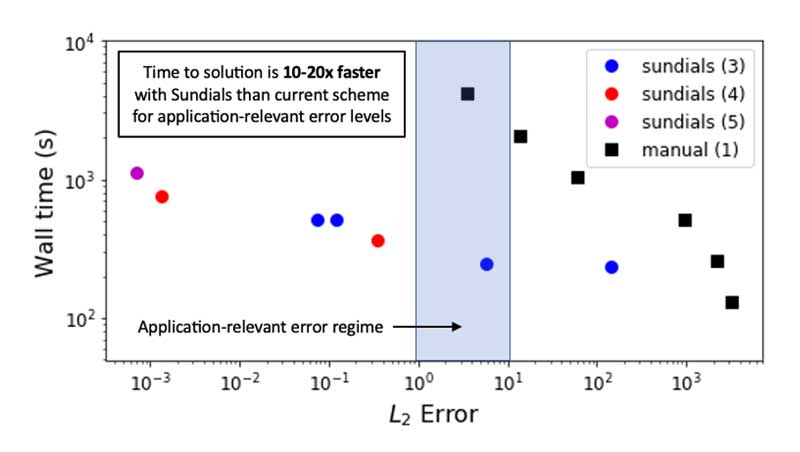
Figure 6. Timing results on the Ascent system for the original MEUMAPPS-SS fixed-step, first-order, time-integration scheme and adaptive, high-order schemes from ARKODE along with the error calculated from a small-time-step reference solution. In the application-relevant error regime, ARKODE is 10×–20× faster than the original scheme when comparing approximate timings at the same error levels. Figure and results are courtesy of Steve DeWitt.

Integration Challenges

The team summarizes the major integration challenges according to two broad categories:

Staying ahead of application needs can be difficult. It requires significant interaction with developers to determine upcoming numerical mathematics and software needs based on physics simulation goals.
Maintaining interfaces can be difficult in the fluid GPU environment.
- System updates, compiler bugs, and other software problems must all be sorted out between libraries and applications.
- With system updates, problems can cause work to stop until both teams can debug simultaneously. This issue highlights the need for collaboration and an ability to communicate quickly.
- Because SUNDIALS sits in the middle of the software stack, the interfaces must work well with components up and down the stack. This issue also reflects the need for a team that has a broad range of software expertise.

The Hypre Project

The ECP hypre project—led by Ulrike Yang (Figure 7), PI and group leader of the mathematical algorithms and computing group and member of LLNL technical staff—focuses on high-performance preconditioners and solvers for solving large, sparse linear systems of equations on massively parallel computers. Hypre can be used to solve many types of linear systems, which can be generated via finite-element or finite-difference methods applied to scalar PDEs (i.e., one unknown per grid point) or systems of PDEs that contain multiple variables per grid point.

Figure 7. Ulrike Meier Yang (left) and GPU experts Rui Li (middle) and Wayne Mitchell (right)

Work on hypre began in the late 1990s. It has since been used by research institutions and private companies to simulate groundwater flow, magnetic fusion energy plasmas in tokamaks and stellarators, blood flow through a heart, fluid flow in steam generators for nuclear power plants, and pumping activity in oil reservoirs, to name a few. In 2007, hypre won an R&D 100 award from R&D World magazine as one of the year’s most significant technological breakthroughs.[12]

A Conceptual Interface

Yang observed, “One of the attractive features of hypre is the provision of conceptual interfaces. These interfaces give application developers a natural means for describing their linear systems and provide access to hypre’s solvers.”

The article, “The Design and Implementation of hypre, a Library of Parallel High Performance Preconditioners,” noted, “These interfaces ease the coding burden and provide extra application information required by certain solvers. For example, application developers who use structured grids typically think of their linear systems in terms of stencils and grids, so an interface that involves stencils and grids is more natural. Such an interface also makes it possible to supply solvers that take advantage of the structured grid. In addition, the use of a particular conceptual interface does not preclude users from building more general sparse matrix structures (e.g., compressed sparse row) and using more traditional solvers (e.g., incomplete LU factorization) that do not use the additional application information.”[13]

The current instantiation of hypre presents several linear system interfaces (Figure 8). For more information, consult the documentation.

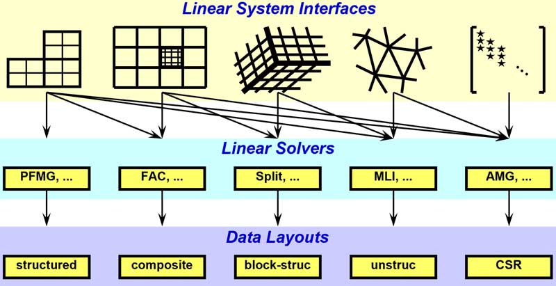
Figure 8. Conceptual linear system interfaces. (Source)

A general hypre workflow consists of first setting up a preconditioner and then calling an iterative solver that uses the preconditioner in each iteration to improve system convergence. The team noted that current architecture trends favor regular computational patterns and large problems to achieve high performance.

A Focus on Multigrid Methods

The general idea that underlies the use of any preconditioning procedure for iterative solvers is to modify a (possibly ill-conditioned) system of equations expressed in matrix form as A*x = b, where A is a large sparse matrix, to obtain an equivalent system for which the iterative method converges faster.[14] Hypre provides several high-performance parallel preconditioners, including multigrid methods.

Multigrid methods are used to find solutions to differential equations by using a hierarchy of discretizations. These discretizations (frequently mapped to a hierarchy of grids that range from coarse to fine) apply to problems that exhibit multiple scales of behavior. The ExaWind project, for example, uses multiple grid resolutions to model entire wind farms (Figure 9).

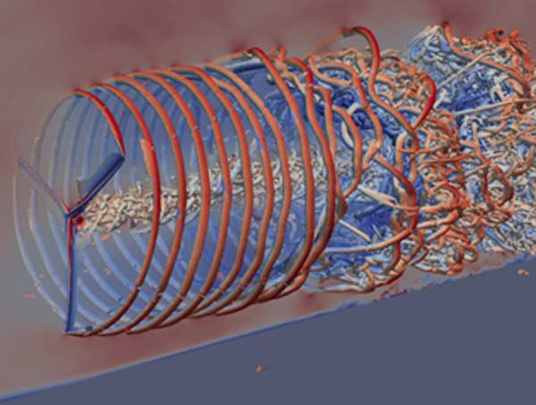
Figure 9. The ExaWind project models entire wind farms by using the hypre BoomerAMG solver, which operates on multiple grid resolutions.

For certain problems, the multigrid approach yields an iterative solver with optimal cost complexity so that the solver can return a solution in a linear number of O(N_DoFs) arithmetic operations.[15]^,[16] The O(N) notation, known as big-O notation, is used to describe how the run time of a system changes according to the problem size denoted by the variable N.

In this case, O(N_DoFs) indicates that the run time varies according to the degrees of freedom in the system, where the degrees of freedom are the number of independent variables that must be specified to determine a solution to the system. On a practical note, Yang clarified, “Multigrid methods of size N can theoretically be solved in O(N) time, but necessary computational overhead—even in a well-designed package—results in a slight increase in runtime to O(N)log(N).” Even when working with large problems, the additional log(N) run time multiplier is not generally considered cost prohibitive.

Hypre supports algebraic multigrid (AMG) methods. These methods construct their hierarchy of operators from the system matrix. They are used to approximate solutions to (sparse) linear systems of equations, and they use the multilevel strategy of relaxation and coarse-grid correction used in traditional geometric multigrid methods. The goal of AMG is to generalize the multilevel process to target problems in which a coarser problem is unapparent—for example, unstructured meshes, graph problems, or structured problems in which uniform refinement is ineffective.[17]

Algebraic multigrid methods deliver both scalability and improved time to solution through preconditioning to achieve fast convergence.

Scalability according to computational nodes: It is often possible to scale the processes (e.g., MPI ranks) with the problem size while achieving similar or slightly longer run times.
Fast time to solution: Preconditioning to achieve fast convergence requires somewhat different approaches that depend on the problem being addressed. For this reason, hypre provides multiple preconditioners and solvers that the user can choose.

Vendor-agnostic support for GPUs is important because hypre resides in the middle of the software stack. The current ECP work focuses on using programming models (e.g., NVIDIA/CUDA, AMD/HIP, and Intel oneAPI/SYCL) so that applications that use hypre can run on all three forthcoming US exascale systems.

A particular challenge with sparse matrix methods is that the computations are, almost without exception, memory-bandwidth limited. Yang observed, “Most users are running hypre’s unstructured methods that operate on sparse matrices. We have spent much effort improving the efficiency of these methods in accessing these data structures. We are happy with our speedups even with the performance limitations of the CPU and GPU memory subsystems.”

Yang noted that the team has addressed both communications and memory-growth issues. Memory utilization, for example, can be an issue because of a potential increase in nonzero entries on coarser levels that results from matrix multiplications. For this reason, hypre uses methods that achieve lower memory overhead through more aggressive coarsening, and this greatly benefits GPU algorithms owing to the smaller on-device memory capacity of these devices.

Sparse matrix methods are an active area of research, and a substantial amount of the literature explores numerous optimization techniques for sparse-matrix calculations—especially on GPUs. Along with leveraging different data structures, the flexibility of the conceptual interface provides the hypre library with the flexibility to incorporate any new advances in the field.

As part of their ECP work, and in support of GPU computing, the team has redesigned some algorithms. For example, the team created new interpolation operators for the AMG solver and preconditioner BoomerAMG ,[18] as highlighted in the ECP website article, “A New Approach in the Hypre Library Brings Performant GPU-Based Algebraic Multigrid to Exascale Supercomputers and the General HPC Community.”

Portable Applications via Different Programming Models

Current computer architectures favor regular computational patterns and large problem sizes, thereby presenting a challenge for unstructured solvers and multigrid methods with decreasing level sizes. The hypre library provides three different interfaces that provide varying degrees of structure and require different porting strategies.

First, the Structured-Grid Interface (Struct) is a stencil-based interface that is most appropriate for scalar finite-difference applications in which the grids consist of unions of logically rectangular (sub)grids (Figure 10). This is an interface that efficiently operates on regular grids.[19] The user defines the matrix and right-hand side in terms of the stencil and the grid coordinates. This geometric description, for example, allows the use of the structured PFMG solver, which is a parallel algebraic multigrid solver with geometric coarsening.

The grid is managed by the box manager, which acts as a distributed directory to the index space that references the boxes.[20] The BoxLoops back end operates on these data structures via macros used to perform loops across the underlying data structures. Back ends that use CUDA, HIP, RAJA, Kokkos, and SYCL provide CPU and multivendor GPU support.

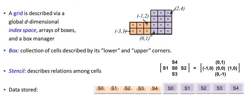
Figure 10. The Struct interface. (Source)

Second, the Semi-Structured-Grid Interface (SStruct) represents a middle ground for GPU efficiency (Figure 11). It is essentially an extension built on the Struct interface, thus leveraging the Struct GPU efficiency while adding some unstructured features (e.g., block-structured, composite, or overset grids).[21] The SStruct interface accommodates multiple variables and variable types (e.g., cell-centered or edge-centered), and that flexibility allows for solving more general problems. This interface requires the user to describe the problem in terms of structured grid parts and then describe the relationship between the data in each part by using either stencils or finite-element stiffness matrices. The hypre team is currently developing a semistructured AMG solver.

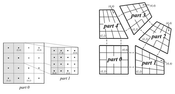
Figure 11. The SStruct interface is a more general interface that leverages the efficiency of the Struct interface on GPUs. (Source)

Third, the Linear-Algebraic Interface (IJ) is a standard linear-algebraic interface that requires users to map the discretization of their equations into row-column entries in a matrix structure. The grid is simply the set of variables, and the coarsening and interpolation processes are determined entirely based on the entries of the matrix. The lack of structure presents serious challenges to achieving high performance on GPU architectures,[22] particularly in designing the parallel coarsening and interpolation algorithms that must combine good convergence and low computational complexity with low memory requirements.[23] BoomerAMG is a commonly used, fully unstructured AMG method built on compressed sparse row matrices. It is used in the ExaWind project.

Exascale Test-Bed Performance

Recent benchmark evaluations demonstrate good performance on the Crusher test bed. Applications that perform well on this test bed reflect well on future performance of the Frontier exascale system due to the identical hardware and similar software between the two systems.

Figure 12 illustrates that the AMD MI250X GPUs deliver significantly faster performance over a range of problem sizes in terms of both setup time and solve time.

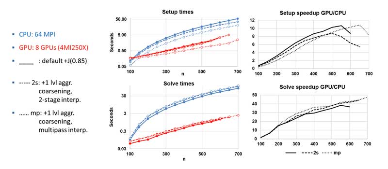
Figure 12. Results for AMG-PCG on one node of Crusher when running a 3D, 27-point diffusion problem on an n³ grid. (Source)

Support the ECP Mission of Exascale Supercomputing

Strong-scaling performance demonstrated by BoomerAMG when running both low- and high-resolution ExaWind simulations on the GPU-accelerated Summit supercomputer reflects well on future exascale performance when there is significant work per device. This trend is highlighted particularly well through the greater number of nodes utilized during the high-resolution run shown in Figure 13.

The benchmark results show the performance when modeling the behavior of two turbines that use an unstructured, unbalanced mesh. The low-resolution results contain 23 million mesh nodes for a single turbine, and the high-resolution results contain 635 million mesh nodes for a single turbine. The key measurements are the average time spent on solving each pressure-Poisson and momentum and scalar transport system of equations. Each simulation operates for 50 timesteps, and the average time per step is reported with error bars. The graphs also include linear regression lines.

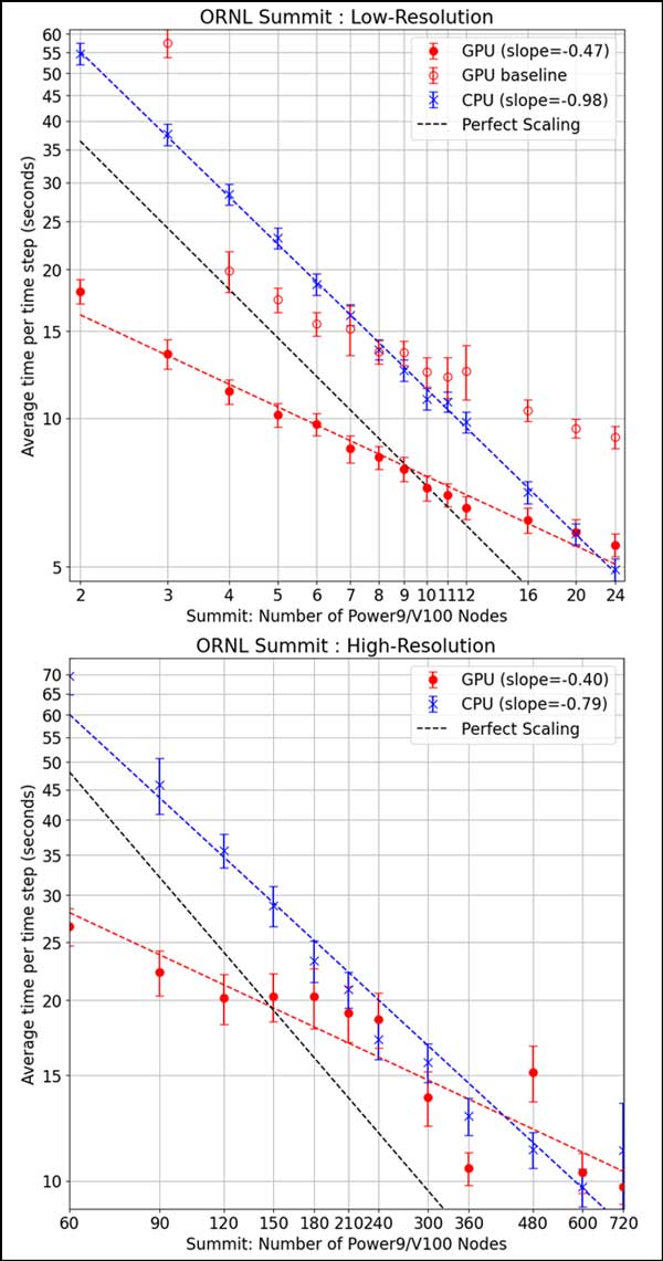
Figure 13. Low- (top) vs. high-resolution strong scaling (bottom) on the Summit supercomputer demonstrated by the ExaWind team. (Source)

Weak-scaling results when using BoomerAMG and the PETSc interface also demonstrate good scaling behavior. Figure 14 reports the weak-scaling results for a Chombo-Crunch computational fluid dynamics (CFD) test on a cylinder packed with microspheres (1,000–25,000 spheres that are 1–32 cm in diameter), and the largest problem represents ~3.2 billion degrees of freedom. Chombo-Crunch adds multicomponent, geochemical reactive transport in complex pore-scale geometry to its CFD model.[24]

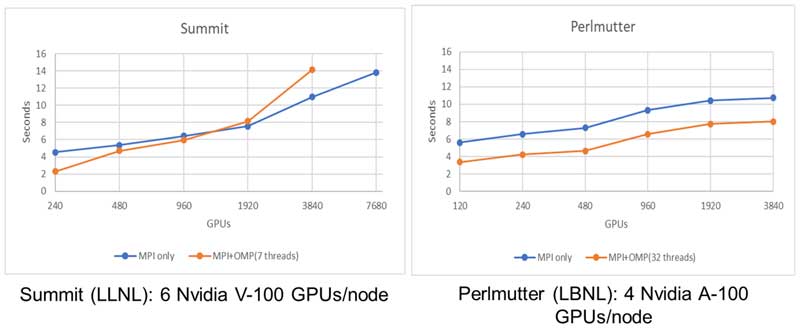
Figure 14. Weak-scaling performance on the Summit (left) and Perlmutter (right) supercomputers.

Summary

The ECP SUNDIALS-hypre project provides two numerical libraries that offer vendor-agnostic, GPU-accelerated performance and CPU support. Both projects employ good software practices to deliver portable performance.

SUNDIALS provides an exascale-capable, adaptive time-step integrator. It supports the deployment and use of SUNDIALS packages within ECP applications through incorporation into the discretization-based codesign centers—AMReX and the Center for Efficient Exascale Discretization—and directly into applications.

Hypre supports multigrid methods on exascale systems. Yang noted, “The hypre team will continue to make efforts to achieve good performance for hypre’s solvers on current and upcoming high-performance computing architectures. The team also focuses on research and development of improved multigrid methods that can solve more difficult problems.”

This research was supported by the Exascale Computing Project (17-SC-20-SC), a joint project of the U.S. Department of Energy’s Office of Science and National Nuclear Security Administration, responsible for delivering a capable exascale ecosystem, including software, applications, and hardware technology, to support the nation’s exascale computing imperative.

Rob Farber is a global technology consultant and author with an extensive background in HPC and in developing machine learning technology that he applies at national laboratories and commercial organizations.

[1] https://www.exascaleproject.org/highlight/a-new-approach-in-the-hypre-library-brings-performant-gpu-based-algebraic-multigrid-to-exascale-supercomputers-and-the-general-hpc-community/

[2] See chapter 4 in CUDA Application Design and Development, https://www.amazon.com/CUDA-Application-Design-Development-Farber/dp/0123884268

[3] https://ieeexplore.ieee.org/abstract/document/7914605

[4] https://libensemble.readthedocs.io/en/develop/platforms/spock_crusher.html

[5] https://docs.olcf.ornl.gov/systems/crusher_quick_start_guide.html

[6] https://en.wikipedia.org/wiki/Ordinary_differential_equation

[7] https://computing.llnl.gov/projects/sundials/uses-sundials

[8] https://computing.llnl.gov/projects/sundials

[9] https://www.exascaleproject.org/reports/

[10] https://www.intel.com/content/dam/develop/external/us/en/documents/the-compute-architecture-of-intel-processor-graphics-gen9-v1d0.pdf

[11] See Table 21 in https://www.exascaleproject.org/wp-content/uploads/2022/02/ECP_AD_Milestone_Map-Applications-to-Target-Exascale-Architecture_v1.0_20210331_FINAL.pdf

[12] https://computing.llnl.gov/projects/hypre-scalable-linear-solvers-multigrid-methods